Maate Not sure I agree with your analysis there ...thus your post is a bit incomplete & a bit biased .
There are a few variances of opinions on a number of things
Suggest you refer to some basis statistical theory ........ but in a different biological context
Refer you to this just to get some basic theory correct as it seems you wouldn't want to
compromise your arguments & statements .
Note I had to cut about 50% of the article out ...as HC said it was just a bit too big
Please refer .....
http://www.wormbook.org/chapters/www_statisticalanalysis/statisticalanalysis.htmlJust for a quick read I've pasted in most of the content save for about the last 6-8 diagrams ands figures . But I reckon you'll demolish the content over a pre dinner glass of plonk
But in summary - it seems that you think IMU's statistical analysis is a bit flawed ...and that's your right to say so - why not just say it rather than try and prove your veneer academic prowess .
Clearly you have too much time on your hands .
And dont bother replying unless the post is at least 10 pages long and had as least 200 references to every salient point . AbstractThe proper understanding and use of statistical tools are essential to the scientific enterprise. This is true both at the level of designing one's own experiments as well as for critically evaluating studies carried out by others. Unfortunately, many researchers who are otherwise rigorous and thoughtful in their scientific approach lack sufficient knowledge of this field. This methods chapter is written with such individuals in mind. Although the majority of examples are drawn from the field of
Caenorhabditis elegans biology, the concepts and practical applications are also relevant to those who work in the disciplines of molecular genetics and cell and developmental biology. Our intent has been to limit theoretical considerations to a necessary minimum and to use common examples as illustrations for statistical analysis. Our chapter includes a description of basic terms and central concepts and also contains in-depth discussions on the analysis of means, proportions, ratios, probabilities, and correlations. We also address issues related to sample size, normality, outliers, and non-parametric approaches.
View attachment 3638792View attachment 3638792
Figure 5. Summary of GFP-reporter expression data for a control and a test group.
Along with the familiar mean and SD,
Figure 5 shows some additional information about the two data sets. Recall that in
Section 1.2, we described what a data set looks like that is normally distributed (
Figure 1). What we didn't mention is that distribution of the data
16 can have a strong impact, at least indirectly, on whether or not a given statistical test will be valid. Such is the case for the
t-test. Looking at
Figure 5, we can see that the datasets are in fact a bit lopsided, having somewhat longer tails on the right. In technical terms, these distributions would be categorized as
skewed right. Furthermore, because our sample size was sufficiently large (n=55), we can conclude that the populations from whence the data came are also skewed right. Although not critical to our present discussion, several parameters are typically used to quantify the shape of the data including the extent to which the data deviate from normality (e.g.,
skewness17,
kurtosis18 and
A-squared19). In any case, an obvious question now becomes, how can you know whether your data are distributed normally (or at least normally enough), to run a
t-test?
Before addressing this question, we must first grapple with a bit of statistical theory. The Gaussian curve shown in
Figure 6A represents a theoretical
distribution of differences between sample means for our experiment. Put another way, this is the distribution of differences that we would expect to obtain if we were to repeat our experiment an infinite number of times. Remember that for any given population, when we randomly “choose” a sample, each repetition will generate a slightly different sample mean. Thus, if we carried out such sampling repetitions with our two populations ad infinitum, the bell-shaped distribution of differences between the two means would be generated (
Figure 6A). Note that this theoretical distribution of differences is based on our actual sample means and SDs, as well as on the assumption that our original data sets were derived from populations that are normal, which is something we already know isn't true. So what to do?
View attachment 3638798View attachment 3638798
Figure 6. Theoretical and simulated sampling distribution of differences between two means.
The distributions are from the gene expression example. The mean and SE (SEDM) of the theoretical (A) and simulated (B) distributions are both approximately 11.3 and 1.4 units, respectively. The black vertical line in each panel is centered on the mean of the differences. The blue vertical lines indicate SEs (SEDMs) on each side.
As it happens, this lack of normality in the distribution of the populations from which we derive our samples does not often pose a problem. The reason is that the distribution of sample means, as well as the distribution of differences between two independent sample means (along with many
20 other conventionally used statistics), is often normal enough for the statistics to still be valid. The reason is the
The Central Limit Theorem, a “statistical law of gravity”, that states (in its simplest form
21) that the distribution of a sample mean will be approximately normal providing the sample size is sufficiently large. How large is large enough? That depends on the distribution of the data values in the population from which the sample came. The more non-normal it is (usually, that means the more skewed), the larger the sample size requirement. Assessing this is a matter of judgment
22.
Figure 7 was derived using a computational sampling approach to illustrate the effect of sample size on the distribution of the sample mean. In this case, the sample was derived from a population that is sharply skewed right, a common feature of many biological systems where negative values are not encountered (
Figure 7A). As can be seen, with a sample size of only 15 (
Figure 7B), the distribution of the mean is still skewed right, although much less so than the original population. By the time we have sample sizes of 30 or 60 (
Figure 7C, D), however, the distribution of the mean is indeed very close to being symmetrical (i.e., normal).
View attachment 3638813View attachment 3638813View attachment 3638831View attachment 3638831View attachment 3638831
Figure 8. Graphical representation of a two-tailed t-test. (A) The same theoretical sampling distribution shown in Figure 6A in which the SEDM has been changed to 5.0 units (instead of 1.4). The numerical values on the x-axis represent differences from the mean in original units; numbers on the green background are values corresponding to the black and blue vertical lines. The black vertical line indicates a mean difference of 11.3 units, the blue vertical lines show SEs (SEDMs). (B) The results shown in panel A are considered for the case where the null hypothesis is indeed true (i.e., the difference of the means is zero). The units on the x-axis represent differences from the mean in SEs (SEDMs). As for panel A, the numbers on the green background correspond to the original differences. The rejection cutoffs are indicated with red lines using ( = 0.05 (i.e., the red lines partition 5% of the total space under the curve on each tail. The blue vertical line indicates the actual difference observed. The dashed blue line indicates the negative value of the observed actual difference. In this case, the two-tailed P-value for the difference in means will be equal to the proportion of the volume under the curve that is isolated by the two blue lines in each tail.
Now recall that The
P-value answers the following question: If the null hypothesis is true, what is the probability that chance sampling could have resulted in a difference in sample means at least as extreme as the one obtained? In our experiment, the difference in sample means was 11.3, where
a::GFP showed lower expression in the mutant
b background. However, to derive the
P-value for the two-tailed
t-test, we would need to include the following two possibilities, represented here in equation forms:
mce-anchorly that the difference is “biologically significant” (i.e., important). A better phrase would be “statistically plausible” or perhaps “statistically supported”. Unfortunately, “statistically significant” (in use often shortened to just “significant”

is so heavily entrenched that it is unlikely we can unseat it. It's worth a try, though. Join us, won't you?
When William Gossett introduced the test, it was in the context of his work for Guinness Brewery. To prevent the dissemination of trade secrets and/or to hide the fact that they employed statisticians, the company at that time had prohibited the publication of any articles by their employees. Gossett was allowed an exception, but the higher-ups insisted that he use a pseudonym. He chose the unlikely moniker “Student”.
15These are measured by the number of pixels showing fluorescence in a viewing area of a specified size. We will use “billions of pixels” as our unit of measurement.
16More accurately, it is the distribution of the underlying populations that we are really concerned with, although this can usually only be inferred from the sample data.
17For data sets with distributions that are perfectly symmetric, the skewness will be zero. In this case the mean and median of the data set are identical. For left-skewed distributions, the mean is less than the median and the skewness will be a negative number. For right-skewed ent.
23Meaning reasons based on prior experience.
ost likely to occur using the Bonferroni method. Thus the Bonferroni method is the most conservative of the approaches discussed, with FDR occupying the middle ground. Additionally, there is no rule as to whether the uniform or non-uniform Bonferroni method will be more conservative as this will always be situation dependent. Though discussed above, ANOVA has been omitted from
Figure 10 since this method does not apply to individual comparisons. Nevertheless, it can be posited that ANOVA is more conservative than uncorrected multiple
t-tests and less conservative than Bonferroni methods. Finally, we can note that the
statistical power of an analysis is lowest when using approaches that are more conservative (discussed further in
Section 6.2).
mce-anchor
| Column 1 |
|---|
| 1 | 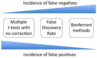 |
|---|
Figure 10. Strength versus weakness comparison of statistical methods used for analyzing multiple means. There is no law that states that all possible comparisons must be made. It is perfectly permissible to choose a small subset of the comparisons for analysis, provided that this decision is made prior to generating the data and not afterwards based on how the results have played out! In addition, with certain datasets, only certain comparisons may make biological sense or be of interest. Thus one can often focus on a subset of relevant comparisons. As always, common sense and a clear understanding of the biology is essential. These situations are sometimes referred to as
planned comparisons, thus emphasizing the requisite premeditation. An example might be testing for the effect on longevity of a particular gene that you have reason to believe controls this process. In addition, you may include some negative controls as well as some “long-shot” candidates that you deduced from reading the literature. The fact that you included all of these conditions in the same experimental run, however, would not necessarily obligate you to compensate for multiple comparisons when analyzing your data.
In addition, when the results of multiple tests are internally consistent, multiple comparison adjustments are often not needed. For example, if you are testing the ability of gene X loss of function to suppress a gain-of-function mutation in gene Y, you may want to test multiple mutant alleles of gene X as well as RNAi targeting several different regions of X. In such cases, you may observe varying degrees of genetic suppression under all the tested conditions. Here you need not adjust for the number of tests carried out, as all the data are supporting the same conclusion. In the same vein, it could be argued that suppression of a mutant phenotype by multiple genes within a single pathway or complex could be exempt from issues of multiple comparisons. Finally, as discussed above, carrying out multiple independent tests may be sufficient to avoid having to apply statistical corrections for multiple comparisons.
mce-anchor3.9. A philosophical argument for making no adjustments for multiple comparisonsImagine that you have written up a manuscript that contains fifteen figures (fourteen of which are supplemental). Embedded in those figures are 23 independent
t-tests, none of which would appear to be obvious candidates for multiple comparison adjustments. However, you begin to worry. Since the chosen significance threshold for your tests was 0.05, there is nearly a 70% chance [1 – (0.95)
23 = 0.693] that at least one of your conclusions is wrong
34. Thinking about this more, you realize that over the course of your career you hope to publish at least 50 papers, each of which could contain an average of 20 statistical tests. This would mean that over the course of your career you are 99.9999999999999999999947% likely to publish at least one error and will undoubtedly publish many (at least those based on statistical tests). To avoid this humiliation, you decide to be proactive and impose a
career-wise Bonferroni correction to your data analysis. From ot include numbers <0% or >100%. Thus, CIs for proportions close to 0% or 100% will often be quite lopsided around the midpoint and may not be particularly accurate. Nevertheless, unless the obtained percentage is 0 or 100, we do not recommend doing anything about this as measures used to compensate for this phenomenon have their own inherent set of issues. In other words, if the percentage ranges from 1% to 99%, use the A-C method for calculation of the CI. In cases where the percentage is 0% or 100%, instead use the exact method.
mce-anchor4.9s of aging and stress, it is common to compare two or more strains for differences in innate laboratory lifespan or in survival following an experimental insult. Relative to studies on human subjects, survival analysis in C. elegans and other simple laboratory organisms is greatly simplified by the nature of the system. The experiments generally begin on the same day for all the subjects within a given sample and the study is typically concluded after all subjects have completed their lifespans. In addition, individual C. elegans rarely need to be censored. That is they don't routinely move way without leaving a forwarding address (although they have been known to crawl off plates) or stop taking their prescribed medicine.One relatively intuitive approach in these situations would be to calculate the mean duration of survival for each sample along with the individual SDs and SEs. These averages could then be compared using a
t-test or related method. Though seemingly straightforward, this dicted nt GM066868.
mce-anchor8. Referencesmce-anchor
Agarwal, P., and States, D.J. (1996). A Bayesian evolutionary distance for parametrically aligned sequences. J. Comput. Biol.
3, 1–17.
AbstractArticlemce-anchor
Agresti, A., and Coull, B.A. (1998). Approximate is better than Exact for Interval Estimation of Binomial Proportions. The American Statistician
52, 119–126.
Articlemce-anchor
Agresti, A., and Caffo, B. (2000). Simple and effective confidence intervals for proportions and differences of proportions result from adding two successes and two failures. The American Statistician
54, 280–288.
Articlemce-anchor
Bacchetti P. (2010). Current sample size conventions: flaws, harms, and alternatives. BMC Med.
8, 17.
AbstractArticlemce-anchor
Benjamini, Y., and Hochberg. Y. (1995). Controlling the false discovery rate: a practical and powerful approach to multiple testing. J. Roy. Statist. Soc. Ser. B Stat. Methodol.
57, pp. 289–300.
Articlemce-anchor
Brown, L.D., Cai, T., and DasGupta, A. (2001). Interval estimation for a binomial proportion. Statist. Sci.
16, 101–133.
Articlemce-anchor
Burge, C., Campbell, A.M., and Karlin, S. (1992). Over- and under-representation of short oligonucleotides in DNA sequences. Proc. Natl. Acad. Sci. U. S. A.
89, 1358-1362.
Abstractmce-anchor
Carroll, P.M., Dougherty, B., Ross-Macdonald, P., Browman, K., and FitzGerald, K. (2003) Model systems in drug discovery: chemical genetics meets genomics. Pharmacol. Ther.
99, 183-220.
AbstractArticlemce-anchor
Doitsidou, M., Flames, N., Lee, A.C., Boyanov, A., and Hobert, O. (2008). Automated screening for mutants affecting dopaminergic-neuron specification in
C. elegans. Nat. Methods
10, 869–72.
Articlemce-anchor
Gassmann, M., Grenacher, B., Rohde, B., and Vogel, J. (2009). Quantifying Western blots: pitfalls of densitometry. Electrophoresis
11, 1845–1855.
Articlemce-anchor
Houser, J. (2007). How many are enough? Statistical power analysis and sample size estimation in clinical research. J. Clin. Res. Best Pract.
3, 1-5.
Articlemce-anchor
Hoogewijs, D., De Henau, S., Dewilde, S., Moens, L., Couvreur, M., Borgonie, G., Vinogradov, S.N., Roy, S.W., and Vanfleteren, J.R. (2008). The
Caenorhabditis globin gene family reveals extensive nematode-specific radiation and diversification. BMC Evol. Biol.
8, 279.
AbstractArticlemce-anchor
Jones, L.V., and Tukey, J. (2000). A sensible formulation of the significance test. Psychol. Methods
5, 411–414.
AbstractArticlemce-anchor
Kamath, R.S., Fraser, A.G., Dong, Y., Poulin, G., Durbin, R., Gotta, M., Kanapin, A., Le Bot, N., Moreno, S., Sohrmann, M., Welchman, D.P., Zipperlen, P., and Ahringer, J. (2003). Systematic functional analysis of the
Caenorhabditis elegans genome using RNAi. Nature
16, 231–237.
AbstractArticlemce-anchor
Knill, D.C, and Pouget, A. (2004). The Bayesian brain: the role of uncertainty in neural coding and computation. Trends Neurosci.
12, 712-719.
AbstractArticlemce-anchor
Nagele, P. (2003). Misuse of standard error of the mean (SEM) when reporting variability of a sample. A critical evaluation of four anaesthesia journals. Br. J. Anaesth.
4, 514-516.
AbstractArticlemce-anchor
Ramsey, F.L. and Schafer, D.W. (2013). The Statistical Sleuth: a Course in Methods of Data Analysis, Third Edition. (Boston: Brooks/Cole Cengage Learning).
mce-anchor
Shaham, S. 2007. Counting mutagenized genomes and optimizing genetic screens in
Caenorhabditis elegans. PLoS One
2, e1117.
Abstractmce-anchor
Suciu, G.P., Lemeshow, S., and Moeschberger, M. (2004). Hand Book of Statistics, Volume 23: Advances in Survival Analysis, N. Balakrishnan and C.R. Rao, eds. (Amsterdam: Elsevier B. V.), pp. 251-261.
mce-anchor
Sulston, J.E., and Horvitz, H.R. (1977). Post-embryonic cell lineages of the nematode,
Caenorhabditis elegans. Dev. Biol.
56, 110–156.
AbstractArticlemce-anchor
Sun, X., and Hong, P. (2007). Computational modeling of
Caenorhabditis elegans vulval induction. Bioinformatics
23, i499-507.
AbstractArticlemce-anchor
Vilares, I., and Kording, K. (2011). Bayesian models: the structure of the world, uncertainty, behavior, and the brain. Ann. N.Y. Acad. Sci.
1224, 22–39.
AbstractArticlemce-anchor
Zhong, W., and Sternberg, P.W. (2006). Genome-wide prediction of
C. elegans genetic interactions. Science
311, 1481–1484.
AbstractArticlemce-anchor9. Appendix A: Microsoft Excel toolsNote: these tools require the Microsoft Windows operating system. Information about running Windows on a Mac (Apple Inc.) can be found at
http://store.apple.com/us/browse/guide/windows.
- PowercalcTool 1mean.xls
- PowercalcTool 2mean.xls
- PowercalcTool prop.xls
- RatiosTool.xls
mce-anchor10. Appendix B: Recomended reading- Motulsky, H. (2010). Intuitive Biostatistics: A Nonmathematical Guide to Statistical Thinking, Second Edition (New York: Oxford University Press).
This is easily my favorite biostatistics book. It covers a lot of ground, explains the issues and concepts clearly, and provides lots of good practical advice. It's also very readable. Some may want more equations or theory, but for what it is, it's excellent. (DF) - Triola M. F., and Triola M.M. (2006). Biostatistics for the Biological and Health Sciences (Boston:Pearson Addison-Wesley).
This is a comprehensive and admirably readable conventional statistical text book aimed primarily at advanced undergraduates and beginning graduate students. It provides many great illustrations of the concepts as well as tons of worked examples. The main author (M. F. Triola) has been writing statistical texts for many years and has honed his craft well. This particular version is very similar to Elementary Statistics (10th edition) by the same author. (DF) - Gonick, L. and Smith, W. (1993). The Cartoon Guide to Statistics (New York: HarperPerennial).
Don't let the name fool you. This book is quite dense and contains the occasional calculus equation. It's an enjoyable read and explains some concepts very well. The humor is corny, but provides some needed levity. (DF) - van Emden, H. (2008). Statistics for Terrified Biologists (Malden, MA: Blackwell Publishing).
This paperback explains certain concepts in statistics very well. In particular, its treatment of the theory behind the T test, statistical correlation, and ANOVA is excellent. The downside is that the author operates under the premise that calculations are still done by hand and so uses many shortcut formulas (algebraic variations) that tend to obscure what's really going on. In addition, almost half of the text is dedicated to ANOVA, which may not be hugely relevant for the worm field. (DF) - Sokal R. R., and Rohlf, F. J. (2012). Biometry: The Principles and Practice of Statisticsin Biological Research, Fourth Edition (New York: W. H. Freeman and Co.).
One of the “bibles” in the field of biostatistics. Weighing in at 937 pages, this book is chock full of information. Unfortunately, like many holy texts, this book will not be that easy for most of us to read and digest. (DF) - Ramsey, F.L. and Schafer, D.W. (2013). The Statistical Sleuth: a Course in Methods of Data Analysis, Third Edition. (Boston: Brooks/Cole Cengage Learning).
Contemporary statistics for a mature audience (meaning those who do real research), done with lots of examples and explanation, and minimal math. (KG) - Fay, D.S., and Gerow, K. (2013). A biologist's guide to statistical thinking and analysis.WormBook, ed. TheC. elegansResearch Community, WormBook,
Quite simply a tour de farce, written by two authors with impeachable credentials and a keen eye for misguiding naïve biologists.
mce-anchor11. Appendix C: Useful programs for statistical calculations- Minitab
A comprehensive and reasonably intuitive program. This program has many useful features and is frequently updated. The downside for Mac users is that you will have to either use a PC (unthinkable) or run it on parallels (or some similar program) that lets you employ a PC interface on your Mac (shudder). (DF) - Microsoft Excel
Excel excels at doing arithmetic, but is not meant to be a statistics package. It does most simple things (t-tests) sort of reasonably well, but the interface is clunky. Minitab (or any other stats package) would be preferred. (KG)
mce-anchor12. Appendix D: Useful websites for statistical calculationsThere are many such sites, which have the advantage of being free and generally easy to use. Of course, what is available at the time of this writing could change rapidly and without notice. As with anything else that's free on the web, rely on at your own risk!
- http://easycalculation.com/statistics/statistics.php
- http://www.graphpad.com/quickcalcs/
- http://stattrek.com/
- http://www.numberempire.com/statisticscalculator.php
- http://www.danielsoper.com/statcalc3/default.aspx
- http://vassarstats.net/
*Edited by Oliver Hobert. Last revised January 14, 2013, Published July 9, 2013. This chapter should be cited as: Fay D.S. and Gerow K. A biologist's guide to statistical thinking and analysis (July 9, 2013),
WormBook, ed. The
C. elegans Research Community, WormBook, doi/10.1895/wormbook.1.159.1,
http://www.wormbook.org.
Copyright: © 2013 David S. Fay and Ken Gerow. This is an open-access article distributed under the terms of the Creative Commons Attribution License, which permits unrestricted use, distribution, and reproduction in any medium, provided the original author and source are credited.


 (20min delay)